

"Cheap" is one of the most abused words in investing, because most people use it to mean a low share price. A stock at $12 feels cheaper than one at $1,200. It isn't — not in any sense that matters. Share price on its own tells you nothing, because it depends entirely on how many slices a company chose to cut itself into. A firm can quadruple its share count in a stock split and leave the business exactly as valuable as before. You want to know how much you are paying for each dollar the business earns or is worth. That is what valuation measures, and there is no single number that settles it. we will walk through three common valuation lenses—the P/E ratio, the PEG ratio, and discounted cash flow, plus the related dividend discount model—and be honest about where each one goes blind.
Before anything else: this guide is general financial education, not investment advice, and nothing in it is a recommendation to buy, sell, or hold any security. Every method here rests on estimates and assumptions that can be wrong, the worked figures are illustrative, and share prices can fall as easily as rise — your capital is at risk. RECATOOLS is not a registered financial adviser. Do your own research and, before you act on any of this, talk to a licensed professional who knows your circumstances.
Two families of answer
Before the individual tools, it helps to sort them. The three-and-a-bit methods here split cleanly into two families that answer different questions. Multiples like the P/E and the PEG are relative. They ask whether a stock is cheap compared to something: its own earnings, its growth rate, its peers. They are fast, they need very little data, and they are the natural first pass. Their weakness is baked into the word "relative": a multiple can tell you a stock is cheaper than its rivals, but not whether the whole peer group is mispriced.
The intrinsic-value models, DCF and the dividend discount model, ask a harder question: what is the business worth on its own, based on the cash it will produce? They give you an absolute number rather than a comparison. The catch is that the number is only as trustworthy as the assumptions you feed in, and those assumptions reach years into a future nobody can see. One family is fast and shallow, the other slow and heavy on assumptions. The sensible approach is to use both and see if they agree.
P/E: the price of a dollar of earnings
The price-to-earnings ratio is the oldest and most quoted of the lot, treated as foundational since Graham and Dodd's Security Analysis. The arithmetic is as simple as it gets: divide a share's market price by the company's earnings per share.
P/E = price per share ÷ earnings per share (EPS)
A P/E of 20 means you are paying $20 for every $1 of annual earnings the company reports. Flip it over and you get the earnings yield — 1 ÷ 20 = 5% — which is the return the earnings represent against today's price. Put a real number through it: a stock at $50 with $2.50 of earnings per share has a P/E of 50 ÷ 2.50 = 20.0, an earnings yield of 5.0%. That is exactly what our P/E ratio calculator returns.
The one wrinkle is which earnings to use. Trailing P/E uses the last twelve months of actual reported EPS — history, already banked. Forward P/E uses forecast EPS for the next twelve months — an estimate, and only as good as the forecaster. A high trailing P/E next to a much lower forward P/E is the market saying it expects earnings to jump; whether that optimism is warranted is a separate question the ratio cannot answer.
P/E's blind spots are the reason no one who knows what they are doing stops here. It ignores growth entirely — a P/E of 30 can be a bargain for a company doubling its profits and a trap for one standing still, and the ratio cannot tell the two apart. It breaks for losses: when EPS is zero or negative the P/E is undefined, and a "negative P/E" carries no information at all, so the whole lens is useless for the loss-making firms that make up much of the market's more exciting end. it is also at the mercy of accounting. A one-off gain, a write-down, a change in depreciation, or a big buyback can skew reported EPS, giving two near-identical companies very different P/Es. Comparing P/Es across unlike sectors compounds the error — utilities and banks structurally trade at lower multiples than fast-growing software, and lining them up side by side is a category mistake rather than an insight.
PEG: bolting growth onto the P/E
The PEG ratio exists to patch P/E's biggest hole — its blindness to growth. Peter Lynch popularised it in One Up on Wall Street, and the idea is intuitive: a high P/E is easier to justify if earnings are growing fast, so divide one by the other.
PEG = P/E ÷ expected annual EPS growth rate
There is a convention here that trips people constantly. The growth rate goes in as the plain percentage number, not the decimal. A stock with a P/E of 20 growing earnings at 20% a year has a PEG of 20 ÷ 20 = 1.0. Divide by 0.20 instead and you get 100, which is nonsense. Our PEG ratio calculator uses the number-in-percent convention, so match it.
Lynch's rule of thumb is that a fairly priced growth company has a PEG of roughly 1 — its P/E about equal to its growth rate. Below 1 may flag a bargain; above 1 may flag a rich price. Treat it as what it is: a seasoned investor's heuristic, not a law of physics. "PEG 0.9, therefore buy" is folk wisdom dressed as arithmetic. Lynch also offered a refinement for dividend payers, the PEGY, which folds the dividend yield into the denominator so income-paying stocks are not penalised for growing more slowly.
PEGY = P/E ÷ (expected growth rate + dividend yield)
A stock with a P/E of 20, growth of 15%, and a 3% dividend yield has a PEGY of 20 ÷ (15 + 3) = 20 ÷ 18 = 1.11 — a touch above Lynch's fair-value line, and a fuller picture than the growth-only PEG of 20 ÷ 15 = 1.33 would give. The calculator will run both.
PEG carries its own warnings, and the tool spells them out. Because you are dividing by growth, the ratio falls apart when growth is near zero — the number explodes toward infinity — and turns meaningless or negative when growth is negative. Worse, the ratio is hostage to which growth number you choose. Historical growth, next year's forecast, and five-year analyst estimates can differ wildly and are often wrong. There is no agreed standard. That ambiguity is not a detail to tidy up later; it is the weakness itself. And because PEG is built on P/E, it inherits every one of P/E's accounting and loss-related problems on top of its own.
DCF: valuing the cash, not the comparison
Discounted cash flow throws out comparison altogether and asks what the business is worth from first principles. The premise is that a company is worth the cash it will hand its owners over its life, with future cash worth less than cash today — a dollar in year seven is worth less than a dollar now, so you discount each future figure back to present value at a rate that reflects the risk. Damodaran's Investment Valuation is the standard modern reference for the mechanics our DCF calculator runs.
The tool uses the common two-stage form. First it projects free cash flow forward for a set number of years, growing it each year, and discounts each year's figure back at the discount rate r. Then, because a company does not stop at year N, it caps the forecast with a terminal value — the worth, as of year N, of every cash flow from year N+1 to forever — using the Gordon growth formula and discounts that back too.
Terminal Value = FCFN · (1 + g) ÷ (r − g), which requires r > g.
That constraint is not a nicety. If the perpetual growth rate g reaches or exceeds the discount rate r, the denominator hits zero or goes negative and the terminal value becomes infinite or absurd, so the calculator enforces r > g and will not let you break it. Add the present values up and you have enterprise value; subtract net debt (total debt minus cash) to get equity value; divide by the share count for a per-share figure.
Enterprise value = Σ PV(FCF) + PV(terminal value) → equity value = EV − net debt → per share = equity value ÷ shares.
Work a clean example to see the machinery. Take free cash flow flat at $100 for five years, a discount rate of 10%, and a terminal growth rate of 2%. The terminal value at year five is 100 · 1.02 ÷ (0.10 − 0.02) = 102 ÷ 0.08 = 1,275. Discount that back over five years: 1,275 ÷ 1.10⁵ = 1,275 ÷ 1.61051 ≈ 791.7. Even in a flat, low-growth case, that discounted terminal value dwarfs the five years of explicit cash flow — which lands us on DCF's central flaw.
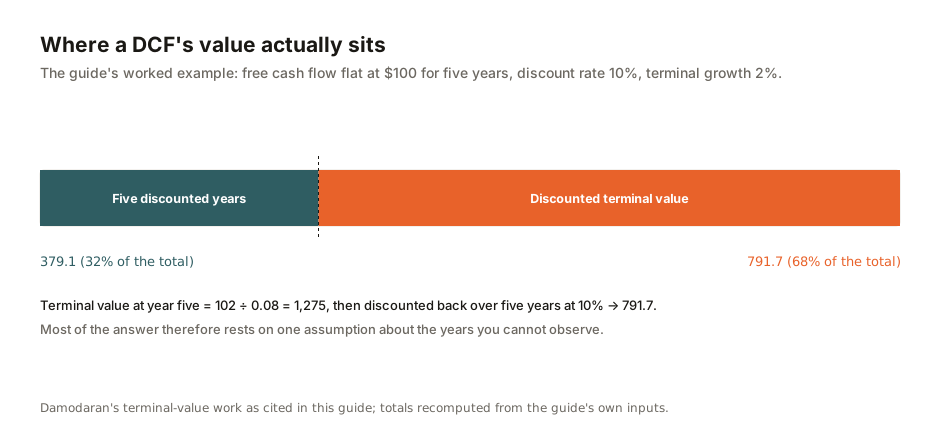
Terminal value routinely makes up well over half of a DCF's total present value, and for a high-growth company far more. Most of your answer, then, rests on a single growth assumption about years you cannot observe. Damodaran named a paper on precisely this problem "The Tail That Wags the Dog?", and he is blunt that of all the inputs to a DCF, none moves the answer more than the stable growth rate — small changes swing the valuation hard, and the effect grows as g approaches r. Our calculator surfaces the terminal value's share of enterprise value for exactly this reason: it tells you how much of the verdict hangs on the least knowable input. There is a discipline on g worth carrying: because no company can outgrow its economy forever, the perpetual growth rate cannot exceed the growth of the wider economy, and a common rule of thumb caps it at the risk-free rate. The old programmer's phrase applies: garbage in, garbage out. A DCF produces a precise-looking number, and that precision is seductive; it is only ever as good as the assumptions behind it, and a motivated analyst can quietly back-solve the inputs to reach whatever answer they wanted.
DDM: DCF for dividend payers
The dividend discount model is DCF with the cash flow narrowed to one thing: the dividend the shareholder actually receives. The constant-growth version, from Myron Gordon's 1959 work, prices a share as next year's dividend divided by the gap between the required return and the dividend growth rate.
P₀ = D₀ · (1 + g) ÷ (r − g) = D₁ ÷ (r − g), again requiring r > g.
Here D₀ is the dividend just paid, D₁ is next year's expected dividend, r is the cost of equity, and g is the constant rate at which the dividend is assumed to grow. Run the numbers our dividend discount model calculator uses: a company that just paid a $2.00 dividend, growing it at 4% a year, with a 9% required return. Next year's dividend is 2.00 · 1.04 = 2.08, and the fair value is 2.08 ÷ (0.09 − 0.04) = 2.08 ÷ 0.05 = $41.60. The calculator also offers a two-stage variant — discount each dividend through an explicit high-growth phase, then apply a Gordon terminal value on the first steady-state dividend — which is structurally the same two-stage machinery as the DCF above, dividends standing in for free cash flow.
The model's honesty is in what it refuses to value. DDM only works for companies that pay a stable, predictable, growing dividend. It is useless for the many firms that pay no dividend at all, and unreliable for high-growth names whose payouts are small, erratic, or plowed back into the business. And it shares the terminal-value model's r > g requirement: get the gap wrong, or let growth meet the required return, and the whole thing collapses.
How the three fit together
None of these is "the" valuation, and treating any one as gospel is the mistake to avoid. The multiples are your fast screens: run a P/E against peers, sanity-check with PEG if the company is growing, and you have a quick read on whether a stock is priced for optimism or for despair. What they cannot tell you is whether the entire comparison set is mispriced — in a bubble, everything looks reasonably valued against everything else. The intrinsic models answer that absolute question, but demand assumptions you cannot verify and repay sloppy inputs with false confidence.
The practical approach is to triangulate. Look at the lenses together, paying attention to where they agree and where they diverge. Convergence raises your confidence without ever proving you right; disagreement is useful, because it points to the specific assumption the market is betting on. The methods are worth using together because they fail in different ways. A stock that looks cheap on every lens is more interesting than one that looks cheap on just one.
| Method | What it needs | Best for | Main blind spot |
|---|---|---|---|
| P/E | Price and EPS (trailing or forward) | A fast relative screen against peers | Ignores growth; undefined when EPS ≤ 0 |
| PEG | P/E plus an expected growth rate | Comparing firms that actually grow | Breaks at zero or negative growth; growth-estimate roulette |
| DCF | FCF forecast, discount rate r, terminal growth g (r > g) | An absolute, cash-based intrinsic value | Terminal value dominates; garbage in, garbage out |
| DDM | A stable growing dividend, cost of equity r, growth g (r > g) | Steady dividend payers | Useless for non-payers and high-growth firms |
- PEG
- 1.00
- Earnings yield
- 5.0%
Growth goes in as a number of percent (20), not a decimal (0.20) — the slip that turns a PEG of 1.0 into 100.
A note for readers in the region
The math is universal — a P/E is computed the same way for an SGX or Bursa Malaysia listing as for one in New York, and none of these formulas change by exchange. Two regional wrinkles are worth knowing, though. Singapore and Malaysia's markets are heavy in banks, REITs, and telcos, sectors that structurally trade on lower multiples and are often valued on dividend yield rather than growth, so a lower average market P/E in Singapore than the US is partly a mix effect, not automatically "cheaper." For REITs in particular, P/E matters less than distribution- and yield-based measures, and a dividend-discount style lens fits them better. And because forward-earnings consensus and analyst growth estimates are thinner for small- and mid-cap ASEAN names than for large US caps, forward P/E and PEG are noisier here — the input, not the formula, is the weak link.
FAQ
Does a lower share price mean a stock is cheaper?
No. Share price alone tells you nothing about value, because it depends on how many shares a company split itself into. A $12 stock is not cheaper than a $1,200 one in any meaningful sense. "Cheap" is about what you pay per unit of earnings or underlying worth — which is what the P/E, PEG, DCF, and DDM lenses are for.
What's the difference between trailing and forward P/E?
Trailing P/E uses the last twelve months of actual reported earnings per share; forward P/E uses the forecast for the next twelve months. Trailing is history you can bank; forward is an estimate that is only as reliable as the forecast behind it. Our P/E ratio calculator computes both.
Is a PEG below 1 always a buy signal?
No. PEG near 1 as "fair value" is Peter Lynch's rule of thumb, not a law of finance. It breaks entirely for near-zero or negative growth, and the answer swings depending on which growth estimate you plug in. Treat a low PEG as one clue among several, not proof.
Why does terminal value matter so much in a DCF?
Because it usually makes up well over half of the total value — for high-growth firms far more. That means most of your answer rests on a single assumption about years you cannot observe. Damodaran called it "the tail that wags the dog?" for a reason. Our DCF calculator shows the terminal value's share of enterprise value so you can see how exposed your valuation is.
When should I use the dividend discount model instead of DCF?
Use the dividend discount model for companies that pay a stable, growing dividend, where the dividend is the cash you actually receive. It is useless for firms that pay no dividend and unreliable for high-growth names with small or erratic payouts — reach for a full DCF or a multiple there instead.
- Aswath Damodaran, Investment Valuation (relative valuation, free-cash-flow/DCF, and dividend-discount-model chapters) — NYU Stern (standard modern reference for P/E mechanics, DCF, and DDM)
- Aswath Damodaran, "Closure in Valuation: Estimating Terminal Value" — NYU Stern (Gordon terminal-value formula, the r > g requirement, and the growth ceiling on g) (accessed 25 Jul 2026)
- Aswath Damodaran, "Terminal Value: The Tail That Wags the Dog?" — NYU Stern (how terminal value dominates a DCF) (accessed 25 Jul 2026)
- Benjamin Graham & David Dodd, Security Analysis — the foundational treatment of the price-to-earnings ratio
- Peter Lynch, One Up on Wall Street (1989) — the PEG ratio, the PEG-near-1 rule of thumb, and the PEGY refinement for dividend payers
- CFA Institute, "Is It Overvalued? Look at the PEG Ratio" — Inside Investing (price multiples and PEG limitations) (accessed 25 Jul 2026)
- Myron J. Gordon (1959), the constant-growth dividend model — the basis of the Gordon-growth DDM