
Twenty test scores go into a spreadsheet. Two lines come out. The first says 87.55 ± 4.36. The second says 87.55 ± 0.97. Nothing was dropped between them. Both are arithmetically correct, both are printed in respectable journals every week, and most readers take them for the same claim written at two levels of precision.
They are not. The larger number is the standard deviation: how far the twenty scores sit from each other. The smaller is the standard error of the mean: how well those scores pin down a single average. One describes the data itself; the other describes your knowledge of its average. Swapping the second for the first divides the printed figure by √20 — a factor of 4.472136 — while the measurements stay exactly as scattered as they were.
We will trace that distinction to the note that tried to fix it in medical publishing, and then turn to our own calculators—which were part of the problem until this morning.

Two numbers, two questions
The dataset is not hypothetical. It is what our standard deviation calculator loads when you press Load sample (20 scores): twenty exam scores between 78 and 95. We ran them through numpy, alongside the quantity the tool does not print.
docker exec w21-sdse python3 /tmp/03-sd-vs-se.py
SEED = 20260725
numpy 2.5.1

PART 1 — the tool's own sample dataset (n=20)
  data      : 85, 92, 78, 95, 88, 90, 82, 87, 93, 80, 91, 86, 89, 84, 88, 92, 85, 90, 87, 89
  n         : 20
  mean      : 87.550000
  SD (pop,  divisor n)   : 4.248235
  SD (samp, divisor n-1) : 4.358597
  SE  = s/sqrt(n)        : 0.974612
  ratio SD/SE            : 4.472136   (= sqrt(n) = 4.472136)
  'mean +/- SD' reads    : 87.55 +/- 4.36   -> 83.19 to 91.91
  'mean +/- SE' reads    : 87.55 +/- 0.97   -> 86.58 to 88.52
  width of the +/-1SD interval : 8.7172
  width of the +/-1SE interval : 1.9492
  SE interval is 22.4% as wide as the SD interval
[…]
If you read the two intervals as claims about the world, they stop being synonyms. The first says most of the class scored between roughly 83 and 92, which a reader can check against the raw list. The second says the class average sits near 87.55, give or take about a point; a reader who takes 86.58 to 88.52 for the range of scores has been misled by a factor of four and a half. The narrower interval is 22.4% as wide as the other — not a finding, just arithmetic on the same twenty numbers.
What Altman and Bland wrote
The cleanest primary statement fits on one page of the BMJ. Douglas Altman and Martin Bland's Statistics Note number 51, "Standard deviations and standard errors" (BMJ 2005;331:903), opens flatly — "The standard deviation (often SD) is a measure of variability" — then draws the line the rest of the literature keeps citing:
"So, if we want to say how widely scattered some measurements are, we use the standard deviation. If we want to indicate the uncertainty around the estimate of the mean measurement, we quote the standard error of the mean."
The link arrives in the same paragraph, stating the whole mechanism: "The standard error of the sample mean depends on both the standard deviation and the sample size, by the simple relation SE = SD/√(sample size)." A sentence later, the consequence: "The standard error falls as the sample size increases, as the extent of chance variation is reduced."
Their practical complaint was about notation. A published "69.4±9.3 kg", they wrote, "gives no indication whether the second figure is the standard deviation or the standard error (or indeed something else)". Their remedy was editorial: the BMJ's policy "is to remove ± signs and request authors to indicate clearly whether the standard deviation or standard error is being quoted. All journals should follow this practice."
To be precise, the note does not accuse anyone of picking the smaller number to flatter a result. That charge exists, and it is quoted below, but it belongs to other authors.
√n is the whole of it
The square root separates the descriptive number from the inferential one, making them behave differently as a study grows. We drew one sample at each of nine sample sizes from a known normal population with μ = 100 and σ = 15, on a single random stream. The sample standard deviation wandered without trending: 12.0820 at n = 4, then 14.8797, 14.0030, 15.4751, 16.7742 at n = 100, and 15.0087 once n reached 100,000. Noisy at the small end, hovering around 15, going nowhere. The standard error on the identical samples fell from 6.0410 to 3.1312 to 1.6774 at n = 100, then 0.4604 at n = 1000 and 0.0475 at n = 100,000. Held against a fixed σ of 15, the substitution shrinks the printed figure to 7.500 at n = 4, 3.000 at n = 25, 1.500 at n = 100 and 0.750 at n = 400 — at a hundred observations, a bar one tenth the size from data of identical variability. Which is why it tempts people who intend no deception: the figure looks tighter, and not one line of the analysis has to change.

Why n−1, and what it does not fix
Before the standard error can be computed, the standard deviation has to be, and the sample version divides by n−1 rather than n — "using n − 1 instead of n in the denominator compensates for the loss of one degree of freedom from estimating the mean µ with X̄", as one open-access preprint states the textbook result. We tested it rather than repeating it: two million replications at each of eight sample sizes on a normal population, and at four more on a skewed exponential one, put the n−1 estimator on the true variance every time — 225.0 for the normal, 100.0 for the exponential.
The convention is called Bessel's correction, and where the name came from we cannot establish. Our own tool page carried a confident origin story, complete with a person and a year, that no primary source we could reach supports. It has been deleted, not swapped for a different guess.
What the correction leaves behind rarely reaches a calculator page. It makes the variance unbiased, not the standard deviation, because a square root is concave.
docker exec w21-sdse python3 /tmp/04-bessel.py
[…]
IMPORTANT CAVEAT — Bessel makes the VARIANCE unbiased, not the SD.
sqrt is concave, so E[sqrt(s^2)] < sqrt(E[s^2]) (Jensen's inequality).

   n | E[s^2] (ddof=1) | E[s] (ddof=1) | c4(n)*sigma | E[s]-sigma
------------------------------------------------------------------
   2 |        225.0624 |       11.9692 |     11.9683 |    -3.0308
   5 |        224.8578 |       14.0945 |     14.0998 |    -0.9055
  10 |        225.0740 |       14.5933 |     14.5899 |    -0.4067
  30 |        224.9439 |       14.8697 |     14.8713 |    -0.1303
 100 |        224.9685 |       14.9611 |     14.9622 |    -0.0389

E[s^2] lands on 225 exactly; E[s] lands BELOW 15 and matches c4(n)*sigma.
So 'divide by n-1' fixes the variance and leaves a residual downward bias
[…]
At n = 100 the residual bias is about 0.25% and nobody need care; at n = 2 the expected sample standard deviation is 11.9692 against a true 15. One correction to our own run: its closing line put the n = 100 bias at "~0.13%", the 1/(8n) form where the first-order term is 1/(4n). That line is elided above; the table is the authority — 14.9611 against a true 15 is 0.26%, and c4(100) = 0.99747798 gives 0.2522%. "Unbiased" is a claim about one quantity, and it does not travel through a square root — which matters, because s is the numerator of every standard error you will ever compute.
One dataset, three legends
The distinction is not academic. We took Group A — the same twenty real scores, mean 87.55 — and a simulated Group B of twenty values, mean 90.576, a gap of 3.0256, then plotted both three times with nothing changed but the legend.
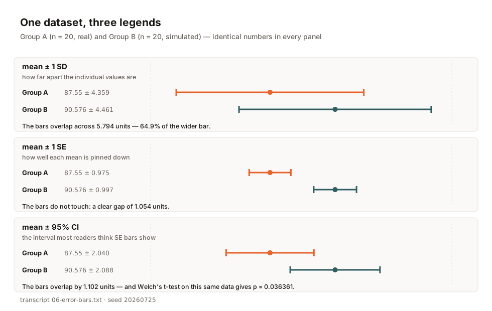
In the first panel the bars sit almost on top of each other, overlapping across 5.794 units — 64.9% of the wider bar — and a reader concludes the groups are indistinguishable. In the second, each has shrunk by a factor of √20 and they no longer touch, leaving a gap of 1.054 units, and the same reader concludes the difference is solid. Neither panel lies. The individual scores do overlap heavily; the two class averages are, separately, well-located.
The third panel is the one worth pinning up. Drawn as 95% confidence intervals — half-widths of 2.040 and 2.088, using t(0.975, 19) = 2.0930 — the bars overlap by 1.102 units. The familiar shortcut—overlapping intervals mean no significant difference—is not a theorem. Here, it gives the wrong answer: Welch's t-test on these numbers returns t = −2.1696 on 37.980 degrees of freedom and p = 0.036361.
| Standard deviation (s) | Standard error of the mean (SE) | |
|---|---|---|
| Question it answers | How far apart are the individual measurements? | How precisely has the mean been estimated? |
| Class of statistic (Cumming et al., Table I) | Descriptive | Inferential |
| As n grows | Settles on a fixed property of the population | Falls toward zero |
| On the twenty-score dataset | 4.358597 | 0.974612 |
| Bar half-width in the figure above | 4.359 (A) / 4.461 (B) | 0.975 (A) / 0.997 (B) |
| SAMPL guideline position | Use it to report variability | Do not use it to report variability |
How often it happens
The first countable rate came from anaesthesia. Peter Nagele's 2003 audit in the British Journal of Anaesthesia reported — in its abstract, as far as we could read, the publisher's full text being closed to us — that "One in four articles (n=198/860, 23%) published in four anaesthesia journals in 2001 inappropriately used the SEM in descriptive statistics to describe the variability of the study sample." The same abstract supplies the motive: "As the SEM is always less than the SD, it misleads the reader into underestimating the variability between individuals within the study sample."
The largest documented rate comes from cardiology, and this one we read in full. Wullschleger and colleagues examined 441 original articles across three cardiovascular journals for 2012 and found 64% — 282 articles — carrying at least one instance of incorrect SEM use. Then the detail that turns a statistics complaint into a reporting problem: "In 81% of articles with incorrect use of SEM, the authors had explicitly stated that they use the SEM for data description and in 89% SEM bars were also used instead of 95% confidence intervals." Not slips. Explicitly stated. Basic science offended at 74% against 10% for clinical work.
There is a counter-signal, however. A 2025 audit of three manual-medicine journals looked at 790 articles, 487 of which reported the SEM, and found inadequate use in just 1.4% of cases, plus 2.5% where the authors never said whether a ± sign meant an SD or an SEM. Its background paragraph sets the wider range: "In medical journals, inappropriate use has been found in 14–64% of articles." One field at 1.4% does not undo three journals at 64%, and its authors do not claim it does.
What the reporting rules say
The bluntest instruction in the reporting literature comes from Altman again, with Thomas Lang, in the SAMPL guidelines hosted by the EQUATOR Network:
"Do NOT use the standard error of the mean (SE) to indicate the variability of a data set. Use standard deviations, inter-percentile ranges, or ranges instead. (The SE is an inferential statistic—it is about a 68% confidence interval—not a descriptive statistic.)"
The capitals are in the original. A page later, SAMPL declines to let the SE stand in as a precision statement either: it "is essentially a 68% confidence coefficient: use the 95% confidence coefficient instead."
This does not make the standard error a bad statistic, a point where many guides of this kind overshoot. Cumming, Fidler and Vaux — the most-cited paper on the subject, and the source of the descriptive/inferential split above — argue the opposite for comparative work. Their fourth rule: "because experimental biologists are usually trying to compare experimental results with controls, it is usually appropriate to show inferential error bars, such as SE or CI, rather than SD." Their complaint is not that people use SE, but that they use it unlabelled, without stating n, then read overlap off the picture as though it settled a test.
The two positions are compatible. If the question is how much the things you measured differ, report a standard deviation, an interquartile range or the range. If it is whether two conditions differ, an inferential bar is the right instrument — and a 95% confidence interval says more, and more honestly, than an SE bar, because its coverage is stated rather than implied.

Our calculators, and what we fixed today
We audited our own statistics tools against these sources before drafting a word, and two failed. As of today, 26 July 2026, both are corrected. The standard deviation calculator labelled its sample standard deviation with the population symbol: both headline boxes read "(σ)", including the one computing s with the n−1 divisor, while a fact card lower down the same page correctly explained the opposite convention. The labels now read s and σ, the variance boxes s² and σ².
A subtler fault sat underneath, of the kind only a rendered page reveals. Those labels carry text-transform: uppercase, which was turning s into S and σ into Σ — so even a correctly written symbol reached the reader as the wrong character. The CSS was collapsing the exact distinction the page exists to teach. Symbols now opt out of the transform on both tools.
The most serious fault on that page was not a label at all. Its parser split on any run of whitespace, comma or semicolon, so a spreadsheet column came apart at its thousands separators: 1,234, 2,500 and 1,750, one per line, entered as six observations — and $1,234.50, $2,500.00 as 234.5 and 500. Every statistic below was then computed correctly on the wrong data, under a placeholder inviting exactly that paste. A comma in 1,234 shape is now read as a thousands separator, not a delimiter, whenever any other delimiter is present.
Downstream, the z-score calculator asks for a population σ and treats whatever arrives as exact, so with its sibling handing over a sample s under a σ label, the error chained. For a value whose true z is 2.00, substituting an s estimated at n = 3 puts the computed z anywhere between 0.90 and 9.18 across the middle 90% of samples; at n = 10, 1.31 to 3.47. Both tools now state what σ has to be. The z tool also printed a significance verdict — a green tick and "Highly significant", or a red cross and "Not significant" — from three inputs that cannot support one. It never asked for n.
docker exec w21-sdse python3 /tmp/05-zscore.py
[…]
PART 3 — the RECATOOLS z-score-calculator defaults, and its missing input
  Tool defaults (z-score-calculator.blade.php lines 55-57 / app.js loadSample):
    x = 85.0, mu = 70.0, sigma = 10.0
    z = (x-mu)/sigma = 1.5000
    two-tailed p     = 0.133614
    the tool prints  : 'Not significant (p >= 0.10)'  [app.js line 89]

  Same numbers, read as a SAMPLE MEAN of n observations instead of one value.
  The test statistic is then (xbar-mu)/(sigma/sqrt(n)) — the SE in the
  denominator, not the SD. The tool has no n field, so it cannot do this.

       n | SE = sigma/sqrt(n) |  z = (xbar-mu)/SE |   two-tailed p | verdict
  --------------------------------------------------------------------------
       1 |            10.0000 |            1.5000 |      1.336e-01 | Not significant (p >= 0.10)
       2 |             7.0711 |            2.1213 |      3.389e-02 | Significant (p < 0.05)
       3 |             5.7735 |            2.5981 |      9.375e-03 | Very significant (p < 0.01)
       4 |             5.0000 |            3.0000 |      2.700e-03 | Very significant (p < 0.01)
       5 |             4.4721 |            3.3541 |      7.962e-04 | Highly significant (p < 0.001)
      10 |             3.1623 |            4.7434 |      2.101e-06 | Highly significant (p < 0.001)
      30 |             1.8257 |            8.2158 |      2.220e-16 | Highly significant (p < 0.001)
[…]
The verdict is removed. The one-tailed and two-tailed figures remain, relabelled as tail areas — which is what they are for a single standardised observation — with a note on why no verdict follows from them. The page's separate accuracy claim survived its check: the worst absolute error against a high-precision reference was about 7×10⁻⁸, inside the advertised ±0.00001.
One part needed no fixing. The three functions we lifted out of the standard deviation calculator's shipped JavaScript — mean, variance and stdDev — were right to the last bit and were left untouched: run under node and cross-checked against numpy, they return 4.358597070279912 and 4.2482349275905165 for the sample and population SD. What failed on that page failed on either side of the arithmetic — at the parser on the way in, and at the labels on the way out.
The third tool needed no repair. Our standard error calculator already put it properly — "It is not the standard deviation of the data itself — that describes spread between individuals. The standard error describes spread between hypothetical replications of the entire study" — and already cited a formula source. It was simply orphaned: neither tool that creates the confusion linked to the one that resolves it. Both now do.
FAQ
Is the standard error just a smaller standard deviation?
No — it is the standard deviation of a different thing. Wullschleger and colleagues put it compactly: "As the sample SD is an estimate of the variability of individual observations, the SEM is an estimate of the variability of the means of different samples."
So should I never report the SEM?
Not that either. SAMPL says do not use it to describe the variability of a dataset, nor as a precision statement in place of a 95% confidence interval. For comparing conditions, though, Cumming, Fidler and Vaux argue inferential bars are usually right, with the interval the more informative. Report the SD when the question is about spread, an interval when it is about a difference, and label whichever you draw.
If two 95% confidence intervals overlap, is the difference not significant?
Not necessarily, and the figure above is a worked counterexample: intervals overlapping by 1.102 units, and a Welch t-test on the identical data returning p = 0.036361. Overlap-by-eye is a rule of thumb about a picture, not a test. Run the test.
Can I put a sample standard deviation into a z-score calculator?
Only when the sample is large enough for the estimate to be stable, and even then a t-based method is the correct route. A nominal 95% interval built on 1.96 with an estimated s actually covers about 81% at n = 3 and 92% at n = 10; the t critical value restores it at every n.
- Altman DG, Bland JM, "Standard deviations and standard errors" — BMJ 2005;331(7521):903 (full text via PubMed Central) (accessed 25 Jul 2026)
- Lang TA, Altman DG, "Basic Statistical Reporting for Articles Published in Biomedical Journals: the SAMPL Guidelines" — EQUATOR Network (PDF) (accessed 25 Jul 2026)
- Cumming G, Fidler F, Vaux DL, "Error bars in experimental biology" — J Cell Biol 2007;177(1):7–11 (accessed 25 Jul 2026)
- Wullschleger M, Aghlmandi S, Egger M, Zwahlen M, "High Incorrect Use of the Standard Error of the Mean (SEM) in Original Articles in Three Cardiovascular Journals Evaluated for 2012" — PLoS ONE 2014;9(10):e110364 (CC BY, full text) (accessed 25 Jul 2026)
- Manovic A, Immelsjö E, Axén I, Palmgren PJ, "Reporting the standard error of the mean: a critical analysis of three journals in manual medicine" — Chiropr Man Therap 2025;33:23 (full text) (accessed 25 Jul 2026)
- Nagele P, "Misuse of standard error of the mean (SEM) when reporting variability of a sample" — Br J Anaesth 2003;90(4):514–516 — abstract only; publisher full text was not reachable, and every Nagele quotation above is from the structured abstract (accessed 25 Jul 2026)
- NIST/SEMATECH e-Handbook of Statistical Methods §1.3.5.6, "Measures of Scale" — the N−1 divisor as printed by NIST (which states the formula but does not argue for it) (accessed 25 Jul 2026)
- "On Bessel's Correction: Unbiased Sample Variance, the Bariance, and a Novel Runtime-Optimized Estimator" — arXiv:2503.22333v5 §3 — un-peer-reviewed preprint, quoted only for its statement of a standard result, which our own simulation reproduces independently (accessed 25 Jul 2026)
- Verification transcripts 03–11 (numpy 2.5.1 / scipy 1.18.0 in a disposable python:3.12-slim container; the tools' own JavaScript under node v22.23.1; RNG seed 20260725 throughout) — run 25 Jul 2026 for this guide

View author profile → · Editorial policy