
Until this morning our own confidence interval calculator printed the sentence this guide exists to correct. Enter a mean, a standard deviation and a sample size, and the result line said we were 95% confident the true population mean lay inside the interval it had just drawn. Lower down the same page, the explainer called that reading a common misinterpretation. One page, two positions, the wrong one in the box the reader actually looks at.
Underneath it sat a second fault, and that one moved the numbers. The tool's table of t-distribution critical values was keyed by a computed tail probability, alpha = (1 - parseFloat(level)) / 2. In IEEE-754 double arithmetic (1 - 0.95) / 2 is 0.025000000000000022, not 0.025, and JavaScript object keys are strings, so the lookup missed at every level the menu offered and every request fell through to a normal-distribution fallback. At n = 5 and 95% the critical-value card read t*(4) = 1.960, where the true figure is 2.7764. The interval it drew was 29.4% too narrow, and an interval built that way covers the population mean 87.799% of the time.
Both faults are fixed as of today, 26 July 2026; the details are further down. We put them at the top because they make the argument in miniature—the label on an interval does not describe how that one interval behaves. Jerzy Neyman wrote the popular reading down in 1937, in the paper that defined the confidence interval, and rejected it in the next sentence.

This guide walks the 1937 paper as written, sets it against a simulation where the true answer is known in advance, and reports what our own calculators were doing about it. The simulation ran on 25 July 2026 in a throwaway container — Python 3.12.13, numpy 2.3.1, scipy 1.16.0, seed 20260725 — and the transcripts appear as they came out.
The sentence Neyman wrote to stop this exact mistake
The confidence interval arrives in print in "Outline of a Theory of Statistical Estimation Based on the Classical Theory of Probability", Philosophical Transactions of the Royal Society A 236(767):333–380. The definition on page 348 names the parts and claims nothing about any one of them: "The functions θ (E) and θ̄ (E) satisfying the above conditions will be called the lower and the upper confidence limits of θ₁. The value α of the probability (20) will be called the confidence coefficient, and the interval, say δ (E), from θ (E) to θ̄ (E), the confidence interval corresponding to the confidence coefficient α."
Further down the same page, Neyman disposes of the idea that a computed interval carries a probability: "In fact, on this assumption, whatever the fixed point E′ and the values θ (E′) and θ̄ (E′), the only values the probability (19) may possess are zero and unity." Zero or one. Nothing between.
The confidence coefficient describes the long-run success rate of the person doing the statistics. On page 349, Neyman puts it this way: "It follows that if the practical statistician applies permanently the rules (a), (b) and (c) for purposes of estimating the value of the parameter θ₁, in the long run he will be correct in about 99 per cent of all cases." Then the detail that rarely survives into a textbook — the repetitions need not be repetitions of the same study. "It is important to notice that for this conclusion to be true, it is not necessary that the problem of estimation should be the same in all the cases." Different parameters, different data, one working life: "Hence the frequency of actually correct statements will approach α."
Neyman then poses and rejects the common misreading. He asks the reader to imagine a finished calculation with limits of 1 and 2, then asks: "Can we say that in this particular case the probability of the true value of θ₁ falling between 1 and 2 is equal to α?" His answer opens the next sentence. "The answer is obviously in the negative. The parameter θ₁ is an unknown constant and no probability statement concerning its value may be made, that is except for the hypothetical and trivial ones". On the same page he likens the theoretical statistician to "the organizer of a game of chance" — the edge belongs to the game, not to the hand you were dealt. (We read page scans of pp. 346–349 only, and make no claim about the rest of the paper.)

What the 95 per cent is a property of
Neyman's claim is testable, and the test costs a few seconds of laptop time. Invent a population whose truth you already know — Normal, mean 100, standard deviation 15 — draw 100,000 independent samples of n = 30 from it, build a 95% t-interval from each in the ordinary way, and count how many contain the number you started with.
seed                     = 20260725
population               = Normal(mu=100.0, sigma=15.0)  <- WE KNOW THE TRUTH
sample size n            = 30
repetitions              = 100,000

========================================================================
PART 1 — long-run coverage of the 95% t-interval
========================================================================
t* critical value (df=29) = 2.045230
intervals built            = 100,000
intervals containing mu    = 95,081
intervals MISSING mu       = 4,919
observed coverage          = 95.081%   (nominal 95%)

========================================================================
PART 2 — the same procedure at other confidence levels
========================================================================
 nominal |        t* |   covered |  observed
----------------------------------------------
   80.0% |    1.3114 |    79,976 |   79.976%
   90.0% |    1.6991 |    89,991 |   89.991%
   95.0% |    2.0452 |    95,081 |   95.081%
   99.0% |    2.7564 |    99,031 |   99.031%
   99.9% |    3.6594 |    99,911 |   99.911%
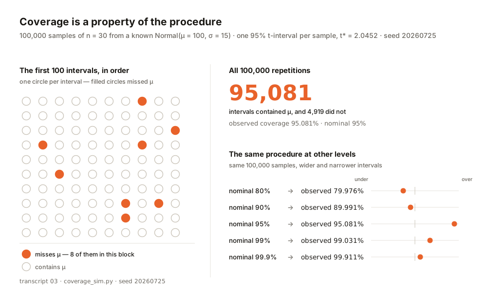
95,081 contained the mean and 4,919 did not: coverage of 95.081% against a nominal 95%. Change the level and the machine tracks it as closely — 79.976% observed at a nominal 80%, 89.991% at 90%, 99.031% at 99%, 99.911% at 99.9%. The critical value at 95% for 29 degrees of freedom is 2.0452, and it is the same 2.0452 for all 100,000 samples. Nothing in the procedure adapts to the data it receives.
The confidence coefficient is nothing more than this: a hit rate for a rule, read from a long run the way a casino reads its own edge. What the run does not say is which intervals were the misses.

One interval at a time, and nothing left to be 95% about
Now stop the run after each draw and look at what you have.
========================================================================
PART 3 — ONE interval at a time: there is no probability left
========================================================================
The first 20 intervals from this run. mu = 100 exactly.
Each interval either contains it or does not. Nothing is 95% about
any single row -- the 95% lives in the column of verdicts.

  # |    x-bar |       s |             95% interval | verdict
----------------------------------------------------------------------
  1 |   95.831 |  14.567 | [  90.3912,  101.2703] | CONTAINS mu
  2 |   96.837 |  15.249 | [  91.1431,  102.5314] | CONTAINS mu
  3 |  105.256 |  15.745 | [  99.3766,  111.1348] | CONTAINS mu
  4 |   97.557 |  16.172 | [  91.5186,  103.5958] | CONTAINS mu
  5 |   98.022 |  16.161 | [  91.9869,  104.0564] | CONTAINS mu
  6 |  100.061 |  17.801 | [  93.4133,  106.7077] | CONTAINS mu
  7 |  101.523 |  13.838 | [  96.3559,  106.6904] | CONTAINS mu
  8 |  107.479 |  16.265 | [ 101.4054,  113.5526] | MISSES mu  <--
…
First interval that MISSES mu is #8: [101.4054, 113.5526]
For that interval, P(mu is inside) is not 0.95 -- it is exactly 0.
For interval #1 [90.3912, 101.2703] it is exactly 1.
Neyman 1937 p.348: the only values that probability may possess
are zero and unity.
…
========================================================================
PART 4 — what a run of 100 intervals looks like
========================================================================
(first 100 intervals; . = contains mu, X = misses)
  .......X.....................X.X.....X............
  ..X.......................X.X.......X.............
misses in this block of 100: 8
The eighth sample came in high, at a sample mean of 107.479, and its interval runs from 101.4054 to 113.5526. The true mean is 100. That interval does not contain it and never did, and no amount of 95% attaches to it. The first interval, 90.3912 to 101.2703, contains the mean with certainty. Identical rule, identical population; what separates the two rows is which sample turned up, and by the time anyone reads the interval, that has already happened.
This is Neyman's "zero and unity" in practice. It is why the popular, wrong sentence cannot be repaired by simply softening the language. Anyone analysing real data is reading row 8 with the verdict column covered up: the run has a known hit rate, this row has an unknown verdict, and those are different facts.
Five ways to misread an interval, numbered
In 2016 Sander Greenland, Stephen Senn, Kenneth Rothman, John Carlin, Charles Poole, Steven Goodman and Douglas Altman published a numbered inventory of statistical misinterpretations in the European Journal of Epidemiology (31:337–350, open access). Twenty-five entries in four groups; items 19 to 23 are the confidence-interval group, printed as declarative statements and then dismantled. Quoted as they appear:
- 19. "The specific 95% confidence interval presented by a study has a 95% chance of containing the true effect size." — the sentence this guide opened with, and the one our own tool printed.
- 20. "An effect size outside the 95% confidence interval has been refuted (or excluded) by the data." — the bounds mark where a rule stopped drawing, not a fence around the possible.
- 21. "If two confidence intervals overlap, the difference between two estimates or studies is not significant." — a comparison neither interval was built to support.
- 22. "An observed 95% confidence interval predicts that 95% of the estimates from future studies will fall inside the observed interval." — the error behind "the next poll should land in this range".
- 23. "If one 95% confidence interval includes the null value and another excludes that value, the interval excluding the null is the more precise one." — precision is width, and width does not depend on where the null sits.
Their own positive statement is narrower: "The 95% refers only to how often 95% confidence intervals computed from very many studies would contain the true size if all the assumptions used to compute the intervals were correct." The conditional is doing real work — the 95,081 above was earned in a simulation where the assumptions held by construction, because we wrote the population ourselves. The American Statistical Association made the parallel point about the neighbouring statistic in March 2016; the second of the six principles in its statement reads, "P-values do not measure the probability that the studied hypothesis is true, or the probability that the data were produced by random chance alone." Same category error, different number.
It is not only students who get this wrong
How widely the misreading is held was measured in a 2014 paper by Rink Hoekstra, Richard Morey, Jeffrey Rouder and Eric-Jan Wagenmakers: "Robust misinterpretation of confidence intervals" (Psychonomic Bulletin & Review 21:1157–1164). Participants read a vignette reporting a 95% confidence interval of 0.1 to 0.4 and marked six statements true or false. Every statement was false: "The questionnaire featured six statements, all of which were incorrect. … Researchers who are aware of the correct interpretation of a CI should have no difficulty checking all 'false' boxes." The sample: "Our sample consisted of 442 bachelor students, 34 master students, and 120 researchers (i.e., PhD students and faculty)."
Item 4 was "There is a 95 % probability that the true mean lies between 0.1 and 0.4." First-year students endorsed it at 58%, master's students at 50%, the researchers at 59%. Item 5 — "We can be 95 % confident that the true mean lies between 0.1 and 0.4." — ran at 49%, 50% and 55%. Seniority did not help, and it was not one slip apiece: "Only 8 first-year students (2 %), no master students, and 3 postmasters researchers (3 %) correctly indicated that all statements were wrong."
The authors printed the statement they had deliberately kept off the questionnaire because it is correct: "If we were to repeat the experiment over and over, then 95 % of the time the confidence intervals contain the true mean." That is transcript 03 in a sentence. Their reason for failing item 5 is the standard our own result line was measured against: "Statements 5 and 6 mention the boundaries of the CI … whereas a CI can be used to evaluate only the procedure and not a specific interval."
Two notes from reading the paper rather than summaries of it. Its participant counts do not reconcile — 442 + 34 + 120 is 596, while the Results section reports 562 participants — so the group figures above are quoted, never a total. And a much-repeated line about respondents endorsing "on average, 2.5 statements" belongs to Oakes's 1986 study of 70 psychologists reading p-values, not to this paper's data.
What our own calculator was printing
This brings us back to our confidence interval calculator. Research for this guide read its shipped source rather than its documentation, ran the real critical-value function inside a disposable Node 22 container, and found that the t-distribution table had never executed once in the life of the page.
=========================================================
B. The alpha the caller actually computes (app.js line 57)
       const alpha = (1 - parseFloat(level)) / 2;
=========================================================
level   | alpha as a JS number      | String(alpha)              | in table?
--------+---------------------------+----------------------------+----------
0.80    | 0.09999999999999998       | 0.09999999999999998        | NO
0.90    | 0.04999999999999999       | 0.04999999999999999        | NO
0.95    | 0.025000000000000022      | 0.025000000000000022       | NO
0.99    | 0.0050000000000000044     | 0.0050000000000000044      | NO
0.999   | 0.0005000000000000004     | 0.0005000000000000004      | NO

(1 - 0.95) / 2 evaluates to 0.025000000000000022 -- not 0.025.
Object keys are strings, so table[0.025000000000000022] is a miss.
The 30-row t-table on app.js lines 34-36 is UNREACHABLE at every
confidence level the UI offers. It has never returned a t value.

=========================================================
C. Where each level actually lands (app.js line 39 fallback)
     return Z_CRIT[(1 - 2*alpha).toFixed(2)] || Z_CRIT['0.95'];
=========================================================
level   | (1-2a).toFixed(2) | Z_CRIT[key] | returned | correct t*(4) | ratio
--------+-------------------+-------------+----------+---------------+-------
0.80    | 0.80              | 1.282       |   1.2820 |        1.5332 | 1.196x
0.90    | 0.90              | 1.645       |   1.6450 |        2.1318 | 1.296x
0.95    | 0.95              | 1.96        |   1.9600 |        2.7764 | 1.417x
0.99    | 0.99              | 2.576       |   2.5760 |        4.6041 | 1.787x
0.999   | 1.00              | undefined   |   1.9600 |        8.6103 | 4.393x

The 99.9% row is the worst: key "1.00" is not in Z_CRIT, so the
|| fallback hands back the NINETY-FIVE percent z, 1.96.
…
=========================================================
E. What the page prints vs what it computed, n=5, 95%
=========================================================
  "Critical value" card shows : t*(4) = 1.960
  interval shown              : [73.6491, 100.5337]
  a real t interval would be  : [68.0499, 106.1329]
  the shown interval is 29.4% too narrow
Section D of the same run confirmed the table's contents were correct all along: called with the literal key 0.025 it returns 2.776 for four degrees of freedom, exactly as a printed table would. Only the lookup was broken. The 99.9% row failed twice over — the fallback key "1.00" is not in the z table either, so the widest interval on the menu came back with the 95% z of 1.96, against a true t*(4) of 8.6103.
Substituting z for t when the standard deviation was estimated from the sample is itself a procedure, with its own coverage. Same 200,000 samples, same nominal level, two rules:
| Sample size | t-interval, labelled 95% | z-interval, labelled 95% | Shortfall |
|---|---|---|---|
| n = 5 | 94.969% | 87.799% | 7.170 pp |
| n = 10 | 94.988% | 91.755% | 3.232 pp |
| n = 30 | 94.973% | 94.044% | 0.929 pp |
| n = 100 | 94.853% | 94.567% | 0.287 pp |
An interval labelled 95%, from a tool that printed t*(4) beside it, covered the mean 87.799% of the time. The gap closes as the sample grows — 0.287 percentage points apart by n = 100, which is where the folk advice that t and z agree for large n comes from. At n = 5 they are 7.170 points apart, and small samples are exactly when someone reaches for a t-interval.
The repair, shipped today, keys the critical-value tables by the confidence-level string from the <select> menu, never by a computed float. An unsupported level now throws an error instead of quietly returning a smaller critical value. Past 30 degrees of freedom the tool interpolates between anchor rows in 1/df rather than dropping to z. The result line now says what the number means — intervals built this way capture the true population mean 95% of the time across repeated samples, and this particular interval either contains it or does not.
The sibling sample size calculator had the sentence right the whole time. Its survey mode tells you to "sample N respondents to estimate the population proportion within ±X percentage points, Y% of the time" — a success rate for a rule, stated as a rate, with no probability attached to any particular survey.
What a margin of error buys
That tool is also where the other half of the trade lives. Survey sizing runs on Cochran's formula, n = z²p(1−p)/e², defaulting to p = 0.5 because p(1−p) is largest there — 385 respondents at 95% confidence and a ±5% margin, against 323 at p = 0.3 and 139 at p = 0.1. Each halving of the margin costs four times the sample, because the margin falls as 1/√n.
When a result sits near a line, read the interval, not just the point estimate. The confidence interval calculator loads a made-up survey by default: 520 yes answers out of 1,000, a sample proportion of 52%. Its Wilson score interval at 95% runs from 0.489018 to 0.550829, and the lower bound is below 0.5. A two-point lead is inside the noise at that sample size, and the tool's own arithmetic says so.
We use the Wilson interval rather than the textbook normal approximation because the approximation's coverage collapses at small proportions. That collapse demonstrates the same general problem in a second statistic. Enumerating every binomial outcome instead of simulating, at n = 20 and a true p of 0.02, the normal-approximation interval labelled 95% covers 33.18% of the time against Wilson's 94.01%. Brown, Cai and DasGupta reached that verdict in Statistical Science 16(2) in 2001: "The performance is so erratic and the qualifications given in the influential texts are so defective that the standard interval should not be used" (§5, p. 117). Their small-sample recommendation is the one our tool follows — "for small n (40 or less), we recommend that either the Wilson or the Jeffreys prior interval should be used" (p. 103).
FAQ
If not 95% probability, what can I say about my interval?
Say what produced it. Hoekstra and colleagues printed the correct form themselves, as the statement they kept off their questionnaire: "If we were to repeat the experiment over and over, then 95 % of the time the confidence intervals contain the true mean." Greenland and colleagues add the condition that makes it true — it holds only if the assumptions used to compute the intervals were correct.
Was our calculator wrong for everyone, or only for small samples?
Every level, at every sample size where the checkbox applied — the tool gated it at n ≤ 30 — the table it was meant to consult was never reached. At four degrees of freedom the understatement ran from 1.196× at 80% to 4.393× at 99.9%; the damage grew with the confidence level, and shrank as the sample grew, because t and z converge.
- Neyman, J. (1937). "Outline of a Theory of Statistical Estimation Based on the Classical Theory of Probability." Philosophical Transactions of the Royal Society A, 236(767), 333–380 — definition and quotations from pp. 348–349 of the journal pagination (accessed 25 Jul 2026)
- Greenland, S., Senn, S. J., Rothman, K. J., Carlin, J. B., Poole, C., Goodman, S. N., & Altman, D. G. (2016). "Statistical tests, P values, confidence intervals, and power: a guide to misinterpretations." European Journal of Epidemiology, 31, 337–350 (open access; PMC4877414) — items 19–23 (accessed 25 Jul 2026)
- Hoekstra, R., Morey, R. D., Rouder, J. N., & Wagenmakers, E.-J. (2014). "Robust misinterpretation of confidence intervals." Psychonomic Bulletin & Review, 21, 1157–1164 (open access) — design and results, pp. 1157–1160 (accessed 25 Jul 2026)
- Wasserstein, R. L., & Lazar, N. A. (2016). "The ASA Statement on p-Values: Context, Process, and Purpose." The American Statistician, 70(2), 129–133; six principles quoted from the ASA release "American Statistical Association Releases Statement on Statistical Significance and P-Values", 7 March 2016, p. 2 (PDF) (accessed 25 Jul 2026)
- Brown, L. D., Cai, T. T., & DasGupta, A. (2001). "Interval Estimation for a Binomial Proportion." Statistical Science, 16(2), 101–133 — recommendations p. 103, standard-interval verdict §5 p. 117 (accessed 25 Jul 2026)
- RECATOOLS transcripts 03, 04, 06, 08 and 09 (25 July 2026) — coverage simulation, z-versus-t coverage, the confidence interval calculator's critical-value code, sample-size scaling, and exact binomial coverage. Python 3.12.13 with numpy 2.3.1 and scipy 1.16.0, and Node v22.23.1, in disposable containers; seed 20260725 wherever randomness was used

View author profile → · Editorial policy